Temporal multilayer network with global relax rates
Data set
Load the 65th multilayer network from the emln package.
This particular network is a temporal plant pollinator multilayer
network without interlayer interactions, and it consists of 6 layers,
corresponding to the flowering season between 2006 and 2011.
library(emln)
# Load multilayer network number 65
emln_65 <- load_emln(65)
## [1] "Creating state node map"
## [1] "Creating extended link list with node IDs"emln_65$layers## # A tibble: 6 × 7
## layer_id latitude location longitude name year layer_name
## <int> <dbl> <chr> <dbl> <chr> <int> <chr>
## 1 1 -32.4 Villavicencio Nature Reserve, Mendoza, Argentina -69.1 all_sites_2006 2006 layer_1
## 2 2 -32.4 Villavicencio Nature Reserve, Mendoza, Argentina -69.1 all_sites_2007 2007 layer_2
## 3 3 -32.4 Villavicencio Nature Reserve, Mendoza, Argentina -69.1 all_sites_2008 2008 layer_3
## 4 4 -32.4 Villavicencio Nature Reserve, Mendoza, Argentina -69.1 all_sites_209 2009 layer_4
## 5 5 -32.4 Villavicencio Nature Reserve, Mendoza, Argentina -69.1 all_sites_2010 2010 layer_5
## 6 6 -32.4 Villavicencio Nature Reserve, Mendoza, Argentina -69.1 all_sites_2011 2011 layer_6head(emln_65$nodes)## # A tibble: 6 × 15
## node_id node_name type corol…¹ corol…² heigh…³ flowe…⁴ body_…⁵ body_…⁶ probo…⁷ probo…⁸ body_…⁹ taxa_…˟ verif…˟ speci…˟
## <int> <chr> <chr> <dbl> <dbl> <dbl> <int> <dbl> <dbl> <dbl> <dbl> <dbl> <chr> <chr> <chr>
## 1 1 aca.ser plant 3.15 0.912 0.154 42118 NA NA NA NA NA TRUE species acanth…
## 2 2 alo.gra plant 5.01 1.02 0.525 5944 NA NA NA NA NA FALSE <NA> aloyss…
## 3 3 arg.sub plant 35.0 28.8 0.514 0 NA NA NA NA NA TRUE species argemo…
## 4 4 arj.lon plant 14.5 1.67 0.222 3252 NA NA NA NA NA TRUE species arjona…
## 5 5 bou.spi plant 10.2 1.48 1.77 1610 NA NA NA NA NA TRUE species bougai…
## 6 6 bre.mic plant 4.17 2 0.32 0 NA NA NA NA NA TRUE species bredem…
## # … with abbreviated variable names ¹corolla_length, ²corolla_aperture, ³height_mean, ⁴flower_abundance,
## # ⁵body_thickness, ⁶body_length, ⁷proboscis_length, ⁸proboscis_width, ⁹body_width, ˟taxa_verified,
## # ˟verification_level, ˟species_namehead(emln_65$extended)## layer_from node_from layer_to node_to weight type
## 1 layer_1 cop.sp2 layer_1 aca.ser 19 pollination
## 2 layer_1 exo.sp1 layer_1 aca.ser 2 pollination
## 3 layer_1 str.eur layer_1 aca.ser 1 pollination
## 4 layer_1 api.mel layer_1 alo.gra 368 pollination
## 5 layer_1 aug.sp layer_1 alo.gra 3 pollination
## 6 layer_1 bom.opi layer_1 alo.gra 5 pollinationInput
A multilayer
link-list format. With this format, a random walker moves within a
layer and with a given relax rate r jumps to another layer
without recording this movement, such that the constraints from moving
in different layers can be gradually relaxed. If the *Inter
exists, then interlayer edges can be used. However, if a relax rate is
also used (Infomap input parameter
--multilayer-relax-rate), the interlayer edges are ignored.
Here we only include *Intra.
# A network in multilayer format
*Intra
#layer node node weight
1 101 1 19
1 113 1 2
1 152 1 1
... some more cases ...
6 69 11 17
6 70 11 2
6 87 11 3
R Code
The description of functions create_multilayer_object
and run_infomap_multilayer in the
infomapecology package contains everything you need to
know. The for loop performs a sensitivity analysis to
examine how structure changes with increasing relax rates.
#Run Infomap and return the network's modular structure at increasing relax-rates.
relaxrate_modules <- NULL
# Initialize an empty data frame to store results
results <- data.frame(relax_rate = numeric(), module_count = numeric())

for (r in seq(0.001,1, by = 0.0999)){
  print(r)
  modules_relax_rate <- run_infomap_multilayer(emln_65, relax = T, silent = T, trials = 50, seed = 497294,    multilayer_relax_rate = r, multilayer_relax_limit_up = 1, multilayer_relax_limit_down = 0, temporal_network = T)
  modules_relax_rate$modules$relax_rate <- r
  relaxrate_modules <- rbind(relaxrate_modules, modules_relax_rate$modules)
  # Append results to the data frame
  results <- rbind(results, data.frame(relax_rate = r, module_count = modules_relax_rate$m))

}
ggplot(results, aes(x = relax_rate, y = module_count)) +
geom_line(color = "blue") +
labs(x = "relax rate (r)", y = "Number of modules")+
theme_bw()+theme(panel.grid.minor = element_blank())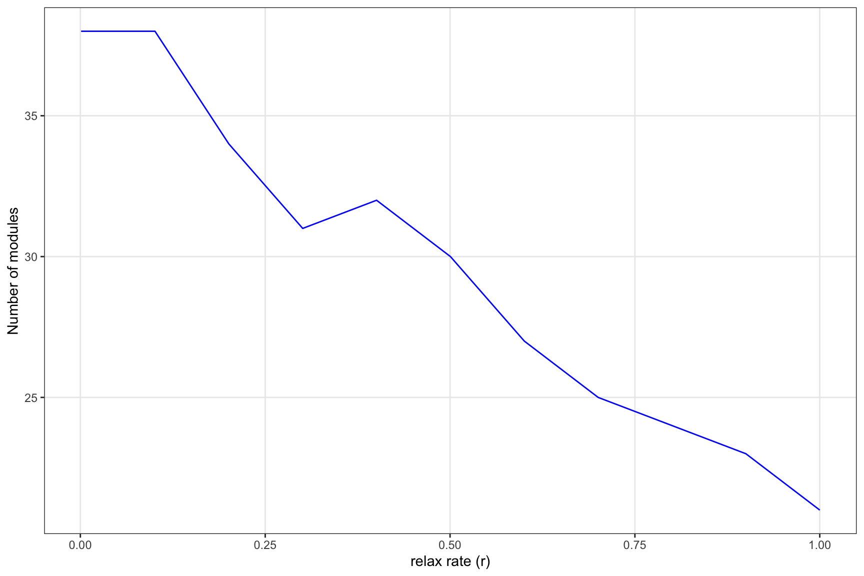
Infomap
Under the hood, the function run_infomap_multilayer
runs:
./Infomap infomap_multilayer.txt . -2 --seed 497294 -N 50 -i multilayer --multilayer-relax-rate 0.15 --multilayer-relax-limit-up 1 --multilayer-relax-limit-down 0 --silentExplanation of key arguments: * -i multilayer indicates
a multilayer input format, which is automatically recognized as a
multilayer link list (and not as a general link list). *
--multilayer-relax-rate 0.15 defines the relax rate (here
0.15). *
multilayer-relax-limit-up 1 --multilayer-relax-limit-down 0
limits relaxation to a single layer upwards (l to l+1), but never
downwards, because time flows one-way.
Output
For multilayer network the output file has a _states
suffix, with the following format. This output is as in Temporal multilayer network with
interlayer edges.
# path flow name stateId physicalId layerId
# path flow name state_id node_id layer_id
1:1 0.0208474 "12" 604 12 6
1:2 0.0166813 "100" 531 100 6
1:3 0.0103777 "45" 600 45 6
1:4 0.00927889 "58" 526 58 6
This output is parsed by run_infomap_multilayer to
obtain a table in which each state node (combination of a physical node
in a layer) is assigned to a module. This can be obtained by (after
running the code above):
#relaxrate_modules$modules
relaxrate_modules %>% select(node_id, layer_id, node_name, type, module, relax_rate)
## # A tibble: 7,062 × 6
## node_id layer_id node_name type module relax_rate
## <int> <int> <chr> <chr> <int> <dbl>
## 1 1 1 aca.ser plant 1 0.001
## 2 1 2 aca.ser plant 10 0.001
## 3 1 3 aca.ser plant 15 0.001
## 4 1 4 aca.ser plant 25 0.001
## 5 1 5 aca.ser plant 31 0.001
## 6 1 6 aca.ser plant 37 0.001
## 7 2 1 alo.gra plant 1 0.001
## 8 2 3 alo.gra plant 16 0.001
## 9 2 4 alo.gra plant 25 0.001
## 10 2 5 alo.gra plant 35 0.001
## # … with 7,052 more rows