Monolayer directed network with hierarchical structure
Example 1
Data set
A binary directed marine food web from Ute et al. 2011. “The Role of Body Size in Complex Food Webs: A Cold Case.” In Advances in Ecological Research, edited by Andrea Belgrano, 45:181–223. Academic Press.. Kongsfjorden is a glacial fjord on the northwest corner of the Svalbard archipelago. It is a 30 km open fjord with no marked sill at the entrance, and with a maximum depth exceeding 300m. The network consists of 262 species with 1,544 feeding interactions. Data is available here.
R Code
# Import data
data("kongsfjorden_links")
data("kongsfjorden_nodes")
nodes <- kongsfjorden_nodes %>%
  select(node_name=Species, node_id_original=NodeID, everything())

interactions<- kongsfjorden_links %>%
  select(from=consumer, to=resource) %>%
  mutate_if(is.factor, as.character) %>%
  mutate(weight=1)

# Prepare network objects
network_object <- create_monolayer_network(x=interactions, directed = T, bipartite = F, node_metadata = nodes)
## [1] "Input: an unipartite edge list"## Warning: One or more rows sum to 0. This may be ok if you expect some links with only outgoing links (e.g., basal species in a food web)## Warning: One or more columns sum to 0. This may be ok if you expect some links with only incoming links (e.g., top predators in a food web)## Joining with `by = join_by(node_name)`# Run infomap, allow hierarchical modules
# Some species will have only incoming or outgoing links, so the next line will result in a warning
infomap_object <- run_infomap_monolayer(network_object, infomap_executable='Infomap',
flow_model = 'directed',
silent=T,trials=100, two_level=F, seed=123)## [1] "Creating a link list..."
## running: ./Infomap infomap.txt . --tree --seed 123 -N 100 -f directed --silent
## [1] "Removing auxilary files..."
Infomap
Under the hood, the function run_infomap_monolayer
runs:
./Infomap infomap.txt . -i link-list --tree --seed 123 -N 100 -f directed --silent- Here, the most important feature is the lack of the
argument
-2(or--two-level), which allows for hierarchical modules (the default in Infomap). -f directedindicates flow on a directed network.
Output
A tree
file is produced by Infomap, but is parsed by
run_infomap_monolayer from infomapecology. In Infomap’s
tree output, the path column has a tree-like format such as
1:3:2, which describes the path from the root of the tree to the leaf
node. The first integer (1 in the 1:3:2 example) is the top module. The
last integer after the colon (2 in the 1:3:2 example) indicates the ID
of the leaf in the module, and not the ID of the node. In case a node
has fewer levels because its module is not partitioned, the missing
levels will show NA.
In the output excerpt below for the analysis of the Kongsfjorden food
web, there are four nodes that belong to the 3rd submodule within top
module 1. For these, module_level3 is the leaf id. Top
modules 2 and 3 do not have sub-modules. Therefore, for these modules
the second level (module_level2) is the leaf id and
module_level3 shows an NA value. In addition,
this data has node attributes, which are added to the final output. In
this example: FeedingType, Mobility and Environment.
| node_id | node_name | module_level1 | module_level2 | module_level3 | FeedingType | Mobility | Environment |
|---|---|---|---|---|---|---|---|
| 54 | Laminaria saccharina | 1 | 1 | 1 | none | 1 | benthic |
| 55 | Laminaria digitata | 1 | 1 | 2 | none | 1 | benthic |
| 57 | Laminaria solidungula | 1 | 1 | 3 | none | 1 | benthic |
| 49 | Fucus distichus | 1 | 1 | 4 | none | 1 | benthic |
| 22 | Calanus finnmarchicus | 1 | 2 | 1 | predator | 4 | pelagic |
| 28 | Metridia lucens | 1 | 2 | 2 | predator | 4 | pelagic |
| 102 | Pandalus borealis | 2 | 2 | NA | predator | 3 | benthic |
| 40 | Thysanoessa inermis | 2 | 3 | NA | grazer | 4 | epipelagic/ice associated |
| 26 | Copepoda nauplii | 3 | 2 | NA | predator | 4 | pelagic |
| 34 | Clione limacina | 3 | 3 | NA | predator | 4 | pelagic |
Example 2
Data set
A binary directed food web from Mouritsen KN, Poulin R, McLaughlin JP, Thieltges DW. Food web including metazoan parasites for an intertidal ecosystem in New Zealand: Ecological Archives E092-173. Ecology. 2011;92: 2006–2006.
In infomapecology:
data(otago_nodes)
data(otago_links)R Code
# Prepare data
otago_nodes_2 <- otago_nodes %>%
  filter(StageID==1) %>%
  select(node_name=WorkingName, node_id_original=NodeID, WorkingName,StageID, everything())
anyDuplicated(otago_nodes_2$node_name)
## [1] 0otago_links_2 <- otago_links %>%
filter(LinkType=='Predation') %>% # Only include predation links
filter(ConsumerSpecies.StageID==1) %>%
filter(ResourceSpecies.StageID==1) %>%
select(from=ResourceNodeID, to=ConsumerNodeID) %>%
left_join(otago_nodes_2, by=c('from'='node_id_original')) %>%
select(from, node_name, to) %>%
left_join(otago_nodes_2, by=c('to'='node_id_original')) %>%
select(from=node_name.x, to=node_name.y) %>%
mutate(weight=1)
# Prepare network objects
# Some species will have only incoming or outgoing links, so the next line will result in a warning
network_object <- create_monolayer_network(x=otago_links_2, directed = T, bipartite = F, node_metadata = otago_nodes_2)## [1] "Input: an unipartite edge list"## Warning: One or more rows sum to 0. This may be ok if you expect some links with only outgoing links (e.g., basal species in a food web)## Warning: One or more columns sum to 0. This may be ok if you expect some links with only incoming links (e.g., top predators in a food web)## Joining with `by = join_by(node_name)`# Run infomap without hieararchy
infomap_object <- run_infomap_monolayer(network_object, infomap_executable='Infomap',
flow_model = 'directed',
silent=T,trials=100, two_level=T, seed=123)## [1] "Creating a link list..."
## running: ./Infomap infomap.txt . --tree --seed 123 -N 100 -f directed --silent --two-level
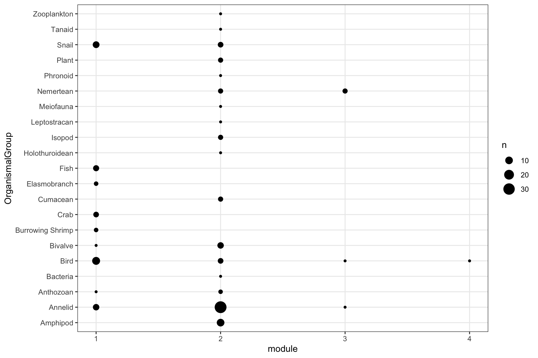
## [1] "Removing auxilary files..."infomap_object$modules %>%
select(node_id, node_name, module=module_level1, OrganismalGroup, NodeType) %>%
group_by(module, OrganismalGroup) %>% summarise(n=n_distinct(node_id)) %>% drop_na() %>%
ggplot(aes(x=module, y=OrganismalGroup, size=n))+geom_point()+
scale_x_continuous(breaks = 1:infomap_object$m)+
theme_bw()+theme(panel.grid.minor = element_blank())## `summarise()` has grouped output by 'module'. You can override using the `.groups` argument.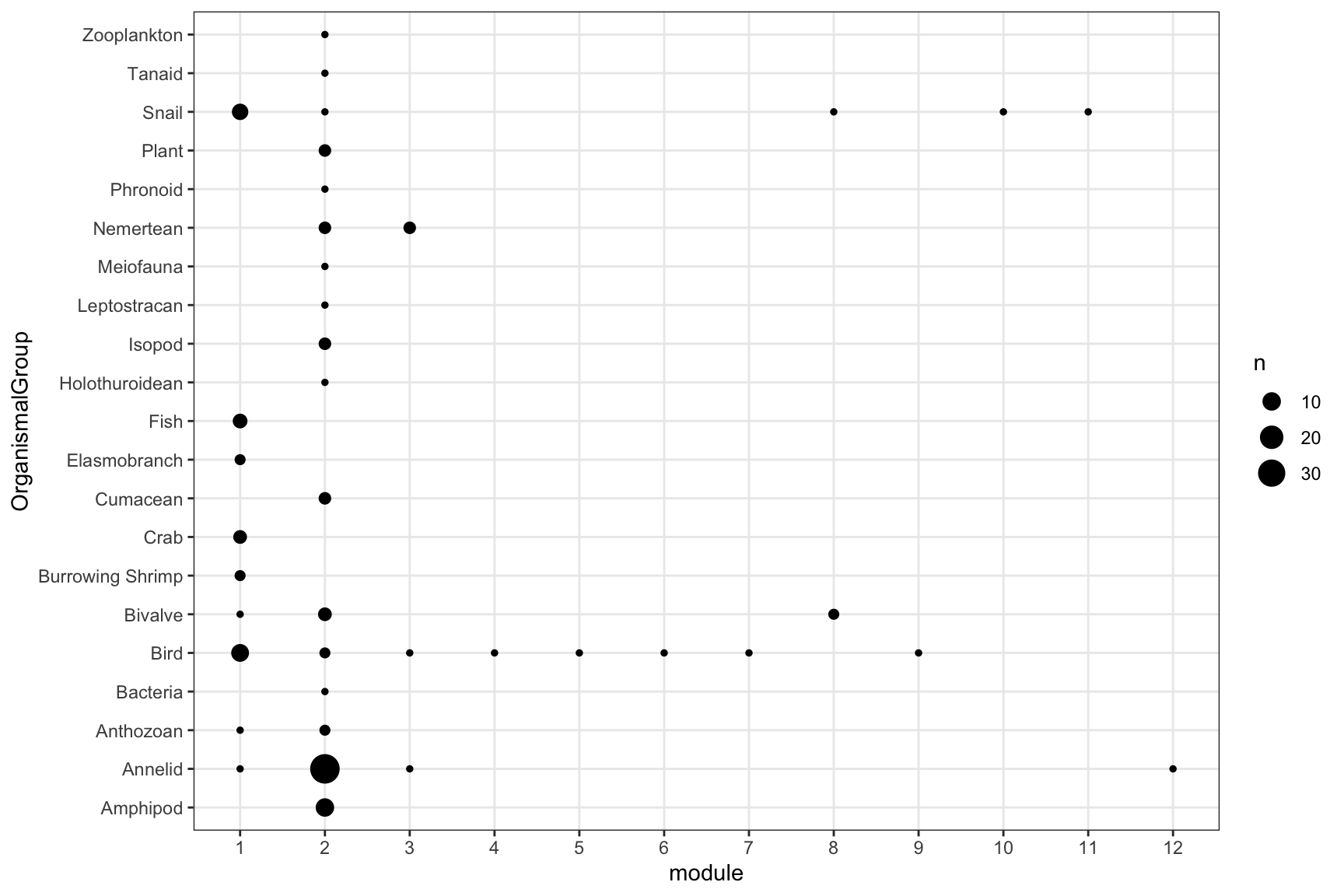
# Run infomap with hieararchy
infomap_object <- run_infomap_monolayer(network_object, infomap_executable='Infomap',
                                        flow_model = 'directed',
                                        silent=T,trials=100, two_level=F, seed=123)
## [1] "Creating a link list..."
## running: ./Infomap infomap.txt . --tree --seed 123 -N 100 -f directed --silent
## [1] "Removing auxilary files..."infomap_object$modules %>%
select(node_id, node_name, module=module_level1, OrganismalGroup, NodeType) %>%
group_by(module, OrganismalGroup) %>% summarise(n=n_distinct(node_id)) %>% drop_na() %>%
ggplot(aes(x=module, y=OrganismalGroup, size=n))+geom_point()+
scale_x_continuous(breaks = 1:infomap_object$m)+
theme_bw()+theme(panel.grid.minor = element_blank())## `summarise()` has grouped output by 'module'. You can override using the `.groups` argument.