Temporal multilayer network with interlayer edges
Data set
A temporal multilayer network. Each layer is a host-parasite bipartite network. Intralayer edges between a parasite species and a host species are the number of parasite individuals divided by the number of host individuals. Interlayer coupling edges connect each physical node to itself in the next layer (e.g., host A in layer 1 to host A in layer 2), and are calculated as the number of individuals in layer l+1 divided by the number of individuals in layer l. They therefore represent population dynamics. Interlayer edges only go one way (l–>l+1) because time flow one way. We represented the undirected edges within each layer as directed edges that go both ways (with the same weight) to be able to have a directed flow. This does not affect the calculation of \(L\). This data set was taken from Pilosof S, Porter MA, Pascual M, Kéfi S. The multilayer nature of ecological networks. Nature Ecology & Evolution. 2017;1: 0101.
Data sets in infomapecology:
The data consists of several matrices representing the host-parasite bipartite network each year, an interlayer extended edge list defining the interlayer links between the same species in different years, and a table containing the attributes of the physical nodes (species).
# Get data
data(siberia1982_matrix)
data(siberia1983_matrix)
data(siberia1984_matrix)
data(siberia1985_matrix)
data(siberia1986_matrix)
data(siberia1987_matrix)
data(siberia_interlayer)
data(siberia_nodes)
Input
An extended multilayer link-list. This multilayer format gives full control of the dynamics, and no other movements are encoded. When using this input format, it is expected that interlayer edges will be provided, otherwise there will be no inter-layer links in the final state network.
*Multilayer
#layer node layer node weight
1 4 1 5 0.1585
1 4 1 6 0.2143
1 4 1 7 0.8276
... some more links...
4 20 4 74 0.0019
4 23 4 10 24.6
4 24 4 5 0.1143
... some more links...
2 16 3 16 1.14285714285714
4 29 5 29 3.66666666666667
5 57 6 57 0.841212121212121
R Code
Because this is a directed bipartite network (interlayer links move from layer to layer in time), we will also consider the intralayer links as directed. To do that, we will convert each bipartite matrix to a symmetric unipartite matrix (see Figure 2, Practical guidelines and the EMLN R package for handling ecological multilayer networks). This does not change the network itself because each link is exactly the same, in both directions.
# Iterate through the layers
for (i in 1982:1987) {
  matrix_data <- get(paste0("siberia", i, "_matrix"))  # Get the matrix by its name

  m <- nrow(matrix_data)
  n <- ncol(matrix_data)

  # Create names for rows and columns
  rcnames <- c(colnames(matrix_data), rownames(matrix_data))

  # Create the square matrix
  square_matrix <- matrix(0, nrow = m + n, ncol = m + n, dimnames = list(rcnames, rcnames))

  # Convert the bipartite matrix to a symmetric unipartite matrix
  # Copy the values from the rectangular matrix into the appropriate positions in the square matrix
  square_matrix[(n + 1):(n + m), 1:n] <- matrix_data
  square_matrix[1:n, (n + 1):(n + m)] <- t(matrix_data)

  # Assign a name to the matrix
  assign(paste0("square_matrix_", i), square_matrix, envir = .GlobalEnv)
}
Now, we will create the multilayer network. Although effectively it
is a bipartite network, we will treat it as an unipartite network to be
able to account for link directions. The description of function
create_multilayer_network is in the package
emln. Plotting is done using two dedicated functions in
infomapecology: plot_multilayer_modules and
plot_multilayer_alluvial.
# Create a multilayer object
layer_attrib <- tibble(layer_id=1:6, layer_name=c('1982','1983','1984','1985','1986','1987'))

multilayer_siberia <- create_multilayer_network(list_of_layers = list(square_matrix_1982,
                                                                      square_matrix_1983,
                                                                      square_matrix_1984,
                                                                      square_matrix_1985,
                                                                      square_matrix_1986,
                                                                      square_matrix_1987),
                                              layer_attributes = layer_attrib,
                                              interlayer_links = siberia_interlayer,
                                              bipartite = F,
                                              directed = T, physical_node_attributes = siberia_nodes )
## [1] "Layer #1 processing."
## [1] "Some nodes have no interactions. They will appear in the node table but not in the edge list"
## [1] "Done."
## [1] "Layer #2 processing."
## [1] "Some nodes have no interactions. They will appear in the node table but not in the edge list"
## [1] "Done."
## [1] "Layer #3 processing."
## [1] "Some nodes have no interactions. They will appear in the node table but not in the edge list"
## [1] "Done."
## [1] "Layer #4 processing."
## [1] "Some nodes have no interactions. They will appear in the node table but not in the edge list"
## [1] "Done."
## [1] "Layer #5 processing."
## [1] "Some nodes have no interactions. They will appear in the node table but not in the edge list"
## [1] "Done."
## [1] "Layer #6 processing."
## [1] "Some nodes have no interactions. They will appear in the node table but not in the edge list"
## [1] "Done."
## [1] "Organizing state nodes"
## [1] "Creating extended link list with node IDs"
## [1] "Organizing state nodes"#Run infomap
multilayer_siberia_modules <- run_infomap_multilayer(M=multilayer_siberia, relax = F, flow_model = 'directed', silent = T, trials = 100, seed = 497294, temporal_network = T)## [1] "Using interlayer edge values to determine flow between layers."
## [1] "./Infomap infomap_multilayer.txt . --tree -2 -N 100 --seed 497294 -f directed --silent"
## [1] "Reorganizing modules..."
## [1] "Removing auxilary files..."
## [1] "Partitioned into 38 modules."#Module persistence
modules_persistence <- multilayer_siberia_modules$modules %>%
group_by(module) %>%
summarise(b=min(layer_id), d=max(layer_id), persistence=d-b+1) %>%
count(persistence) %>%
mutate(percent=(n/max(multilayer_siberia_modules$module$module))*100)
# 1. Modules' persistence
plot_multilayer_modules(multilayer_siberia_modules, type = 'rectangle', color_modules = T)+
scale_x_continuous(breaks=seq(0,6,1))+
scale_y_continuous(breaks=seq(0,70,5))+
scale_fill_viridis_c()+
theme_bw()+
theme(panel.grid.major = element_blank(),
panel.grid.minor = element_blank(),
axis.title = element_text(size=20),
axis.text = element_text(size = 20),
legend.text = element_text(size=15),
legend.title = element_text(size=20))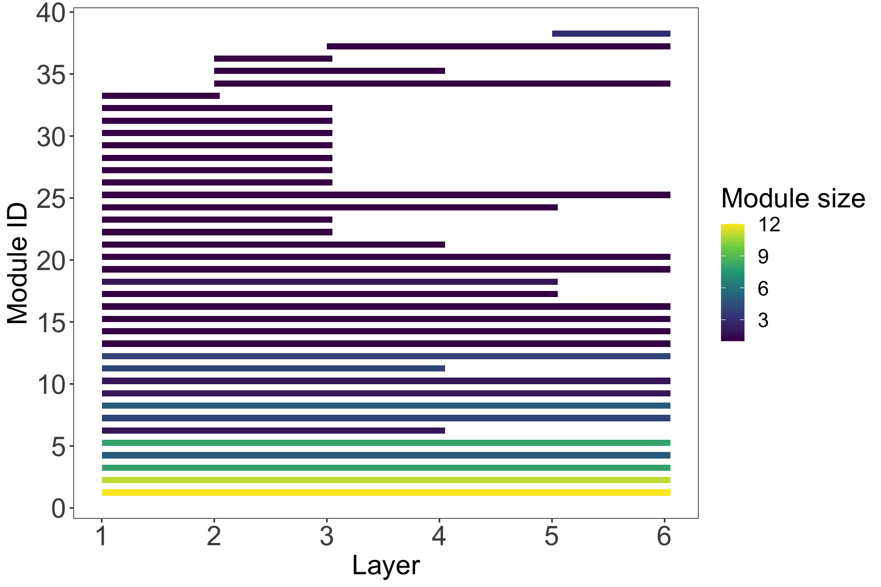
#2. Species flow through modules in time
plot_multilayer_alluvial(multilayer_siberia_modules, module_labels = F)+
  scale_x_continuous(breaks=seq(0,6,1))+
  scale_y_continuous(breaks=seq(0,70,5))+
  labs(y='Number of species')+
  theme_bw()+
  theme(legend.position = "none",
        panel.grid = element_blank(),
        axis.text = element_text(color='black', size = 20),
        axis.title = element_text(size=20))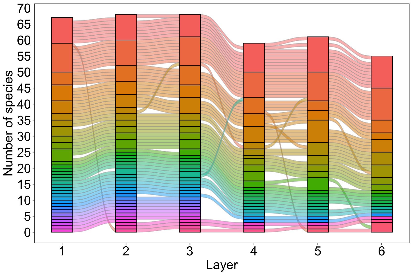
Infomap
Under the hood, the function run_infomap_multilayer
runs:
./Infomap infomap_multilayer.txt . -2 --seed 497294 -N 100 -i multilayer -f directed --silentExplanation of key arguments: * -i multilayer indicates
a multilayer input format, which is automatically recognized as a general
multilayer link-list. * -f directed indicates flow on a
directed network. The visitation rates of nodes is obtained with a
PageRank algorithm based on the direction and weight of edges. This
includes interlayer edges.
Output
For multilayer network the output file has a _states
suffix, with the following format. Note the state_id column. For
example, node 6 in layer 5 has a state_id of 377 (last line). The
state_ids are created by Infomap but not used in our R code.
# path flow name state_id node_id layer_id
1:1 0.0350053 "7" 334 7 6
1:2 0.0294496 "7" 205 7 4
1:3 0.0291166 "7" 280 7 5
1:4 0.0283014 "7" 137 7 3
1:5 0.0124629 "7" 69 7 2
1:6 0.00734334 "7" 3 7 1
1:7 0.00180819 "33" 171 33 3
         ...
11:1 0.00929888 "52" 328 52 6
11:2 0.00861513 "52" 272 52 5
11:3 0.00694999 "52" 211 52 4
11:4 0.00564292 "52" 146 52 3
11:5 0.00256943 "52" 76 52 2
11:6 0.00101397 "52" 14 52 1
12:1 0.0083305 "16" 340 16 6
         ...
This output is parsed by run_infomap_multilayer to
obtain a table in which each state node (combination of a physical node
in a layer) is assigned to a module. This can be obtained by:
multilayer_siberia_modules$modules %>% select(node_id, layer_id, node_name, type, module)## # A tibble: 378 × 5
## node_id layer_id node_name type module
## <int> <int> <chr> <chr> <int>
## 1 1 1 Amalaraeus_penicilliger paras 2
## 2 1 2 Amalaraeus_penicilliger paras 2
## 3 1 3 Amalaraeus_penicilliger paras 2
## 4 1 4 Amalaraeus_penicilliger paras 2
## 5 1 5 Amalaraeus_penicilliger paras 2
## 6 1 6 Amalaraeus_penicilliger paras 2
## 7 2 1 Amerosejus_corbicula paras 22
## 8 2 2 Amerosejus_corbicula paras 22
## 9 2 3 Amerosejus_corbicula paras 22
## 10 3 1 Amphipsylla_sibirica paras 19
## # … with 368 more rows