Example for EMLN analysis
library(emln)
library(tidyverse)
library(infomapecology)
library(magrittr)
The emln package is a valuable tool for importing,
storing, and converting multilayer network data. In this section, we
will demonstrate its practical application for downstream analysis using
examples: (1) node-level analysis using an imported data set, and (2) a
mesoscale analysis using a package-included data set.
We emphasize that the goal of the following analyses is purely technical. We do not assume to study or interpret results in the data sets we use in the example.
Node-level analysis with an imported dataset
At this analysis level, we will compare the eigenvector centrality
scores for each state node when calculated separately per layer (as in a
monolayer network), to those calculated in the multilayer. We use the
get_igraph function to get the individual layers and the
get_sam function of EMLN to get the supra-adjacency matrix
(SAM) to get the multilayer.
This comparison aims to highlight the differences between monolayer and multilayer representations. Since eigenvector centrality takes into account the entire network’s structure when calculating the centrality of each node, we anticipate no correlation. Examining the scores in different contexts (mono vs multilayer) offers valuable insights and alternative perspectives on node importance.
Creating a Multilayer Object
Before calculating the eigenvector centrality scores for each state
node, it is recommended to transform the data into a multilayer object
using the create_multilayer_network function. This
facilitates the handling of the data and ensures a smoother analysis
process.
We use the data from Kefi et al 2016. The data represents a node-aligned multiplex network consisting of three layers: trophic interactions, non-trophic positive interactions, and non-trophic negative interactions. For detailed instructions on creating a multilayer object, please refer to the Example with real data from Kefi 2016 section. The files are also available on our repository (file: website_kefi_data.zip).
# Load and organize the trophic interactions matrix
chilean_TI <- read_delim('chilean_TI.txt', delim = '\t')
nodes <- chilean_TI[,2]
names(nodes) <- 'Species'
chilean_TI <- data.matrix(chilean_TI[,3:ncol(chilean_TI)])
dimnames(chilean_TI) <- list(nodes$Species,nodes$Species)

# Load and organize the negative non-trophic interactions matrix
chilean_NTIneg <- read_delim('chilean_NTIneg.txt', delim = '\t')
nodes <- chilean_NTIneg[,2]
names(nodes) <- 'Species'
chilean_NTIneg <- data.matrix(chilean_NTIneg[,3:ncol(chilean_NTIneg)])
dimnames(chilean_NTIneg) <- list(nodes$Species,nodes$Species)

# Load and organize the negative non-trophic positive matrix
chilean_NTIpos <- read_delim('chilean_NTIpos.txt', delim = '\t')
nodes <- chilean_NTIpos[,2]
names(nodes) <- 'Species'
chilean_NTIpos <- data.matrix(chilean_NTIpos[,3:ncol(chilean_NTIpos)])
dimnames(chilean_NTIpos) <- list(nodes$Species,nodes$Species)


layer_attributes <- tibble(layer_id=1:3, layer_name=c('TI','NTIneg','NTIpos'))
multilayer_kefi <- create_multilayer_network(list_of_layers = list(chilean_TI,chilean_NTIneg,chilean_NTIpos),
                                             interlayer_links = NULL,
                                             layer_attributes = layer_attributes,
                                             bipartite = F,
                                             directed = T)
## [1] "Layer #1 processing."
## [1] "Done."
## [1] "Layer #2 processing."
## [1] "Some nodes have no interactions. They will appear in the node table but not in the edge list"
## [1] "Done."
## [1] "Layer #3 processing."
## [1] "Some nodes have no interactions. They will appear in the node table but not in the edge list"
## [1] "Done."
## [1] "Creating extended link list with node IDs"
## [1] "Organizing state nodes"Eigenvector Centrality
We will now calculate the eigenvector centrality score of each state node using the two different methods:
Method 1: Monolayer Context
Calculating the Eigenvector centrality score of each state node on a per-layer basis.
# get a list of igraph objects as layers igraph
g_layer <- get_igraph(multilayer_kefi, bipartite = F, directed = T)

# get Eigenvector scores of igraph layers
eigen_igraph = c()
for (layer in g_layer$layers_igraph){
  eigen_igraph <- append(eigen_igraph, igraph::eigen_centrality(layer, scale = T)$vector)
}
Method 2: Multilayer Context
Calculating the eigenvector centrality score of each state node using a SAM of the multilayer network.
# get the SAM
sam_multilayer <- get_sam(multilayer = multilayer_kefi, bipartite = F, directed = T, sparse = F, remove_zero_rows_cols = F)

# converting SAM to igraph object
graph_sam <- graph_from_adjacency_matrix(sam_multilayer$M,mode = "directed",weighted = NULL,diag = TRUE,add.colnames = NULL,add.rownames = NA)

# get Eigenvector scores
eigen_sam <- igraph::eigen_centrality(graph_sam, directed = T, scale = T)$vector
Results
We visualize the correlation between the two sets of scores using a
scatter plot. The scatter plot was created by merging the scores into a
data frame called ec_comparison and using the
ggplot2 package. The x-axis and y-axis represent the
multilayer and monolayer scores, respectively. The function
geom_abline() adds a reference line to the scatter plot.
Nodes that fall on this line have the same score in a monolayer and a
multilayer context.
# merge to data frame eigenvector comparison
ec_comparison <- data.frame(eigen_sam, eigen_igraph)
colnames(ec_comparison) <- c("multilayer","monolayer")

# scatter plot using r ggplot2
ggplot(data = ec_comparison, aes(monolayer, multilayer)) +
           geom_point(color = "blue", size = 0.75) +
           labs(title = "Eigenvector Centrality (EC) comparison", x = "EC (monolayer)", y = "EC (multilayer)")+
  geom_abline()+
  scale_x_continuous(limits = c(0,1))+
  scale_y_continuous(limits = c(0,1))+
  coord_fixed() +
  theme_bw()+
  theme(panel.grid.major = element_blank(),
        panel.grid.minor = element_blank(),
        axis.title = element_text(size=15),
        axis.text = element_text(color='black',size = 10),
        legend.text =  element_text(size=15),
        legend.title = element_text(size=20))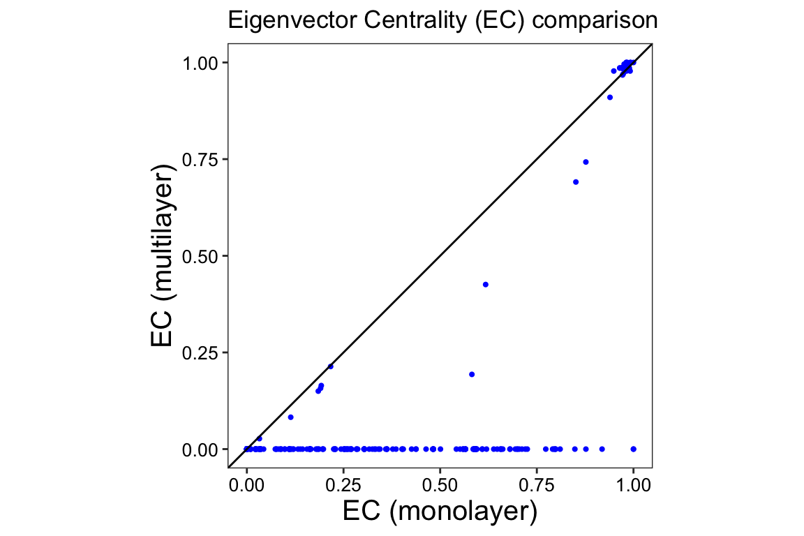
The deviation of the points from the reference line indicates a lack of correlation between the two centrality scores. We see that the majority of the nodes that are important in a monolayer, lose this importance in the multilayer network. There is also a group of species that are important in both network types (upper right corner). This highlights the value of considering the unique ecological processes and interactions represented by different layers when analyzing multilayer networks and interpreting node importance.
Mesoscale level analysis with included data sets
In this example, we showcase how to load and analyze a data set
included in the emln package. At the mesoscale level of
network analysis, examining network properties such as modularity can
provide insights into the temporal behavior of species communities. In
this analysis, we use the community detection algorithm
infomap with the infomapecology
package to detect modules in a temporal multilayer network.
Loading the data
To begin, we load network number 65 using the load_emln
function, which returns a multilayer object.
emln_65 <- load_emln(65)## [1] "Creating state node map"
## [1] "Creating extended link list with node IDs"emln_65$layers## # A tibble: 6 × 7
## layer_id latitude location longitude name year layer_name
## <int> <dbl> <chr> <dbl> <chr> <int> <chr>
## 1 1 -32.4 Villavicencio Nature Reserve, Mendoza, Argentina -69.1 all_sites_2006 2006 layer_1
## 2 2 -32.4 Villavicencio Nature Reserve, Mendoza, Argentina -69.1 all_sites_2007 2007 layer_2
## 3 3 -32.4 Villavicencio Nature Reserve, Mendoza, Argentina -69.1 all_sites_2008 2008 layer_3
## 4 4 -32.4 Villavicencio Nature Reserve, Mendoza, Argentina -69.1 all_sites_209 2009 layer_4
## 5 5 -32.4 Villavicencio Nature Reserve, Mendoza, Argentina -69.1 all_sites_2010 2010 layer_5
## 6 6 -32.4 Villavicencio Nature Reserve, Mendoza, Argentina -69.1 all_sites_2011 2011 layer_6emln_65$nodes## # A tibble: 180 × 15
## node_id node_name type corolla_length corolla_aperture height_mean flower_abundance body_thickness body_length proboscis_length proboscis_width
## <int> <chr> <chr> <dbl> <dbl> <dbl> <int> <dbl> <dbl> <dbl> <dbl>
## 1 1 aca.ser plant 3.15 0.912 0.154 42118 NA NA NA NA
## 2 2 alo.gra plant 5.01 1.02 0.525 5944 NA NA NA NA
## 3 3 arg.sub plant 35.0 28.8 0.514 0 NA NA NA NA
## 4 4 arj.lon plant 14.5 1.67 0.222 3252 NA NA NA NA
## 5 5 bou.spi plant 10.2 1.48 1.77 1610 NA NA NA NA
## 6 6 bre.mic plant 4.17 2 0.32 0 NA NA NA NA
## 7 7 bud.men plant 5.46 1.19 0.49 301 NA NA NA NA
## 8 8 cap.ata plant 0.25 1.69 1.61 59 NA NA NA NA
## 9 9 cen.sol plant 17.5 1.5 0.122 3 NA NA NA NA
## 10 10 cer.arv plant 5.27 13.3 0.277 480 NA NA NA NA
## # ℹ 170 more rows
## # ℹ 4 more variables: body_width <dbl>, taxa_verified <chr>, verification_level <chr>, species_name <chr>head(emln_65$extended)## layer_from node_from layer_to node_to weight type
## 1 layer_1 cop.sp2 layer_1 aca.ser 19 pollination
## 2 layer_1 exo.sp1 layer_1 aca.ser 2 pollination
## 3 layer_1 str.eur layer_1 aca.ser 1 pollination
## 4 layer_1 api.mel layer_1 alo.gra 368 pollination
## 5 layer_1 aug.sp layer_1 alo.gra 3 pollination
## 6 layer_1 bom.opi layer_1 alo.gra 5 pollinationThis is a temporal plan-pollinator multilayer network with
nrow(emln_65$layers) layers and
max(emln_65$nodes$node_id) physical nodes. The network
comprises nrow(emln_65$extended) intralayer edges that are
directed and weighted, with no interlayer interactions.
Community detection (modularity) analysis
Next, we use infomap with infomapecology to
detect modules. We first prepare the data for analysis by selecting the
relevant columns and modifying their names. Then, we run
infomap on the modified data set, considering factors such
as relaxation rate and limits.
Note that the function create_multilayer_object
prepares a multilayer object for infomapecology. Future
versions of infomapecology will directly use the multilayer
object created by the EMLN package.
emln_65_modularity <- run_infomap_multilayer(M = emln_65,
                                               relax = T, silent = TRUE,
                                               trials = 50, seed = 497294,
                                               multilayer_relax_rate = 0.15,
                                               multilayer_relax_limit_up = 1,
                                               multilayer_relax_limit_down = 0,
                                               temporal_network = T)
## [1] "Using global relax to determine flow between layers."
## [1] "./Infomap infomap_multilayer.txt . --tree -2 -N 50 --seed 497294 --silent --multilayer-relax-rate 0.15 --multilayer-relax-limit-up 1 --multilayer-relax-limit-down 0"
## [1] "Reorganizing modules..."
## [1] "Removing auxilary files..."
## [1] "Partitioned into 38 modules."Let’s take a look at the modules.
# Number of modules:
emln_65_modularity$m
## [1] 38emln_65_modularity$modules %>%
select(node_id, layer_id, node_name, type, module)## # A tibble: 642 × 5
## node_id layer_id node_name type module
## <int> <int> <chr> <chr> <int>
## 1 1 1 aca.ser plant 1
## 2 1 2 aca.ser plant 13
## 3 1 3 aca.ser plant 16
## 4 1 4 aca.ser plant 4
## 5 1 5 aca.ser plant 4
## 6 1 6 aca.ser plant 36
## 7 2 1 alo.gra plant 1
## 8 2 3 alo.gra plant 7
## 9 2 4 alo.gra plant 4
## 10 2 5 alo.gra plant 34
## # ℹ 632 more rowsModule persistence
As this is a temporal network, we can observe module persistence and its temporal dynamics. we plot the changes in each module’s size over time.
# Module' persistence
plot_multilayer_modules(emln_65_modularity, type = 'rectangle', color_modules = T)+
  scale_x_continuous(breaks=seq(0,6,1))+
  scale_y_continuous(breaks=seq(0,40,5))+
  scale_fill_viridis_c()+
  theme_bw()+
  theme(panel.grid.major = element_blank(),
        panel.grid.minor = element_blank(),
        axis.title = element_text(size=20),
        axis.text = element_text(size = 20),
        legend.text =  element_text(size=15),
        legend.title = element_text(size=20))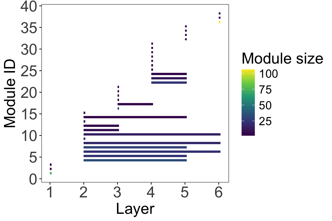
Note that in the first layers there are 4 modules that do not persist. Than, in the second layer modules emerge that persist, some until the 6th layer.
We can also visualize the modular structure over time by plotting the species flow through modules. In this visualization, modules are represented by colors, the size of rectangles indicates the number of species in each module, and curved lines depict species moving between layers (time periods).
# Species flow through modules in time
plot_multilayer_alluvial(emln_65_modularity, module_labels = F)+
  scale_x_continuous(breaks=seq(0,6,1))+
  scale_y_continuous(breaks=seq(0,150,20))+
  labs(y='Number of species')+
  theme_bw()+
  theme(legend.position = "none",
        panel.grid = element_blank(),
        axis.text = element_text(color='black', size = 20),
        axis.title = element_text(size=20))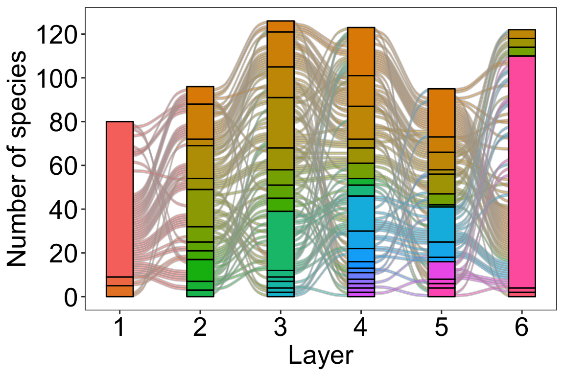
This visual representation of how species transition between modules over time helps us gain insights into the dynamics of species communities.
For more details on temporal multilayer network analysis using
infomapecology visit Temporal
multilayer network with global relax rates and Temporal
multilayer network with interlayer edges.